ExceL vba でプログラミング

エラー

on error next

えらーが検出されても次の行に進む

onerror goto 0
の行まで有効

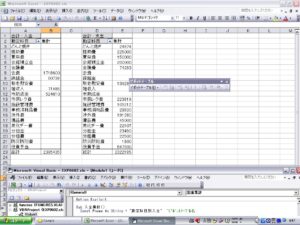
エラーが検出されるとぴポットテーブルを削除

pivottotablewizardメソッド
sourcetype:集合元ノデータxldatabase
sourcedata:集計に使用するデータ
tabledestination:配置場所

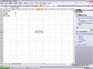
表側項目の指定
addfieldメソド：rowfields 勘定科目

集計項目

orientation  テーブルフィールド
name  合計：入金
function  合計

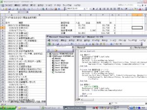
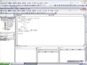
Option Explicit

Sub 入金集計()
Const Pname As String = “勘定科目別入金”  ‘ﾋﾟﾎﾞｯﾄﾃｰﾌﾞﾙ名

‘過去に作成したﾋﾟﾎﾞｯﾄﾃｰﾌﾞﾙを削除する。
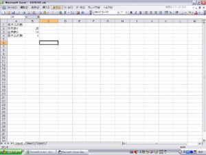
Worksheets(“科目別集計”).Activate
On Error Resume Next
‘ﾃｰﾌﾞﾙが存在しないとエラーになる。
ActiveSheet.PivotTables(Pname).PivotSelect “”, xlDataAndLabel
‘エラーでないときのみセレクションをクリア
If Err.Number = 0 Then Selection.Clear
On Error GoTo 0

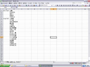
Worksheets(“元帳”).Activate
‘ SourceDataは、キー入力マクロで作成すると”元帳!R3C1:R191C7″のような
‘ 文字列指定になりますが、プログラミングではRangeで与えたほうが楽です。
ActiveSheet.PivotTableWizard _
SourceType:=xlDatabase, _
SourceData:=Cells(3, 1).CurrentRegion, _
TableDestination:=”科目別集計!R1C1″, _
TableName:=Pname

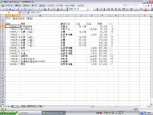
ActiveSheet.PivotTables(Pname).AddFields RowFields:=”勘定科目”
With ActiveSheet.PivotTables(Pname).PivotFields(“入金”)
.Orientation = xlDataField
.Name = “合計 : 入金”
.Function = xlSum
End With
End Sub

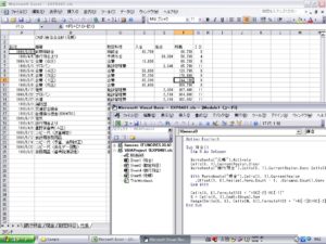
Sub 出金集計()
Const Pname As String = “勘定科目別出金”  ‘ﾋﾟﾎﾞｯﾄﾃｰﾌﾞﾙ名

Worksheets(“科目別集計”).Activate
On Error Resume Next
ActiveSheet.PivotTables(Pname).PivotSelect “”, xlDataAndLabel
If Err.Number = 0 Then Selection.Clear
On Error GoTo 0

Worksheets(“元帳”).Activate
ActiveSheet.PivotTableWizard _
SourceType:=xlDatabase, _
SourceData:=Cells(3, 1).CurrentRegion, _
TableDestination:=”科目別集計!R1C4″, _
TableName:=Pname

ActiveSheet.PivotTables(Pname).AddFields RowFields:=”勘定科目”
With ActiveSheet.PivotTables(Pname).PivotFields(“出金”)
.Orientation = xlDataField
.Name = “合計 : 支出”
.Function = xlSum
End With
End Sub

 

勘定科目の昇順にデータソート
subtotal メソッド　グループ集計
Group by パラメータは　対象列
Function パラメタ　集計方法　xlsum
TotalList パラメタ対象列４列目と５列目同時
Array(4,5)
Replace パラメタ　既存の集計表と置き換え(true)
PageBreaks パラメタ　改ページを挿入しない(False)
SummaryBlowData 集計行を詳細データのしたに表示する(true)

 

Sub 集計()
Worksheets(“元帳”).Activate
勘定科目ソート
Cells(4, 1).CurrentRegion.Select
Selection.Subtotal GroupBy:=3, Function:=xlSum, TotalList:=Array(4, 5), _
Replace:=True, PageBreaks:=False, SummaryBelowData:=True
End Sub

Private Sub 勘定科目ソート()
Worksheets(“元帳”).Activate
Cells(4, 1).CurrentRegion.Select
Selection.Sort Key1:=Range(“C4”), Order1:=xlAscending, Header:=xlGuess, _
OrderCustom:=1, MatchCase:=False, Orientation:=xlTopToBottom, SortMethod _
:=xlPinYin
End Sub

Sub 解除()
‘   SubTotalの解除
Worksheets(“元帳”).Activate
Cells(4, 1).CurrentRegion.RemoveSubtotal

日付ソート
End Sub

Private Sub 日付ソート()
Worksheets(“元帳”).Activate
Cells(4, 1).CurrentRegion.Select
Selection.Sort Key1:=Range(“A4”), Order1:=xlAscending, Header:=xlGuess, _
OrderCustom:=1, MatchCase:=False, Orientation:=xlTopToBottom, SortMethod _
:=xlPinYin
End Sub

 

勘定科目ソート

key:=Range(“C4”) 第一優先キーは勘定科目
Order1:=xlAsending 第一優先キーの並び順は昇順
Header:=xlGuess 見出しの有無はデータに依存

日付ソート

勘定科目ソート

key:=Range(“Ａ4”) 第一優先キーは日付
Order1:=xlAsending 第一優先キーの並び順は昇順
Header:=xlGuess 見出しの有無はデータに依存

 

Sub 勘定科目ソート()
Worksheets(“元帳”).Activate
Cells(4, 1).CurrentRegion.Select
Selection.Sort Key1:=Range(“C4”), Order1:=xlAscending, Header:=xlGuess, _
OrderCustom:=1, MatchCase:=False, Orientation:=xlTopToBottom, SortMethod _
:=xlPinYin

End Sub

Sub 日付ソート()
Worksheets(“元帳”).Activate
Cells(4, 1).CurrentRegion.Select
Selection.Sort Key1:=Range(“A4”), Order1:=xlAscending, Header:=xlGuess, _
OrderCustom:=1, MatchCase:=False, Orientation:=xlTopToBottom, SortMethod _
:=xlPinYin

End Sub

選択併合

private su sheetmarge(sname as string)

snameはサブルーチんが呼び出されるときに実際の
値が確定。
sub プロシージャーは２回呼び出される。
１度目は銀行預金シート
２度目は現金シート
dp1 dp2 はモジュール全体で有効

Option Explicit
Dim Dp1 As Integer      ‘元帳を追加する行番号を保持
Dim Dp2 As Integer      ‘手持金を追加する行番号を保持
Const Sp As Integer = 4   ‘定数を定義。追加する際の先頭の行番号

Sub 併合()
Worksheets(“元帳”).Cells(3, 1).CurrentRegion.Offset(1, 0).Clear
Dp1 = Sp  ‘4行目から記入

Worksheets(“手持金”).Cells(3, 1).CurrentRegion.Offset(1, 0).Clear
Dp2 = Sp  ‘4行目から記入

SheetMarge “銀行預金”
SheetMarge “現金”
End Sub

Private Sub SheetMarge(sName As String)
Dim Ep As Integer, Cc As Integer

Worksheets(sName).Activate
Ep = Cells(Sp, 1).End(xlDown).Row
For Cc = Sp To Ep
If Cells(Cc, 3).Value = “手持ち金” Then
With Worksheets(“手持金”)
Range(Cells(Cc, 1), Cells(Cc, 7)).Copy .Cells(Dp2, 1) ‘.Paste
If Dp2 = Sp Then    ‘もし先頭行なら
.Cells(Dp2, 6).FormulaR1C1 = “=RC[-2]-RC[-1]”
Else
.Cells(Dp2, 6).FormulaR1C1 = “=R[-1]C+RC[-2]-RC[-1]”
End If
Dp2 = Dp2 + 1
End With
Else
With Worksheets(“元帳”)
Range(Cells(Cc, 1), Cells(Cc, 7)).Copy .Cells(Dp1, 1) ‘.Paste
If Dp1 = Sp Then    ‘もし先頭行なら
.Cells(Dp1, 6).FormulaR1C1 = “=RC[-2]-RC[-1]”
Else
.Cells(Dp1, 6).FormulaR1C1 = “=R[-1]C+RC[-2]-RC[-1]”
End If
Dp1 = Dp1 + 1
End With
End If
Next Cc
End Sub

 

併合

■CurrentRegionプロパティ
あるセルを起点としてデータの連続領域を返す。

■copy メソッド
引数がない場合はコピー元のオブジェクトをクリップボードにコピー。
引数がセルの場合は、セルにコピーする。

■Resize
resize(rowsize,columnsize)
指定されたセル範囲をかえす。

■cells(3,1).end(xldown).offset(1,0)
セル(3,1)の終端行End(xldown)の次の行
offset(1,0)をコピー先に

Option Explicit

Sub 併合()
Dim N As Integer

Worksheets(“元帳”).Activate
Cells(3, 1).CurrentRegion.Clear
Worksheets(“銀行預金”).Cells(3, 1).CurrentRegion.Copy Cells(3, 1)

With Worksheets(“現金”).Cells(3, 1).CurrentRegion
.Offset(1, 0).Resize(.Rows.Count – 1, .Columns.Count).Copy Cells(3, 1).End(xlDown).Offset(1, 0)
End With

Cells(4, 6).FormulaR1C1 = “=RC[-2]-RC[-1]”
N = Cells(4, 1).End(xlDown).Row
Range(Cells(5, 6), Cells(N, 6)).FormulaR1C1 = “=R[-1]C+RC[-2]-RC[-1]”
End Sub

 

関数を自分で宣言し、利用する。最大公約数マクロを、Imax関数として宣言しこれを引用する。

－－－－－－－－－－－－－－－－－－

Sub マクロ3()
Dim I As Long, J As Long, W As Long
I = Cells(2, 2).Value
J = Cells(3, 2).Value

Cells(4, 1).Value = “最大公約数”
Cells(4, 2).Value = Imax(I, J)
End Sub

Function Imax(ByVal Ii As Long, ByVal Jj As Long) As Long
Dim W As Long
While Ii <> 0
If Ii < Jj Then
W = Ii
Ii = Jj
Jj = W
End If
Ii = Ii Mod Jj
Wend
Imax = Jj
End Function

Ｅxcel sheetを作る

フォームを作成

ラベル・テキストボックス・リストボックス・コマンドボタン

 

イベントプロシジャーの作成

 

Option Explicit
——————–
Private Sub UserForm_Initialize()
‘リストボックスへのデータ表示
ListBox1.List = Sheets(“勘定科目”).Range(“B1:B23”).Value
‘月日の初期値
TextBox1.Text = Year(Now())
TextBox2.Text = Month(Now())
TextBox3.Text = Day(Now())
End Sub
——————–
Private Sub CommandButton2_Click()
‘［終了］ボタンクリック時の処理
Unload UserForm1
End Sub
———————–
Private Sub CommandButton1_Click()
Dim R As Integer
‘レコード出力位置の検出
R = Cells(3, 1).End(xlDown).Row + 1
‘フォームデータをセルに出力する
Cells(R, 1).Value = TextBox1.Text & “/” & TextBox2.Text & “/” & TextBox3.Text
Cells(R, 1).NumberFormatLocal = “yyyy/m/d”
Cells(R, 2).Value = TextBox4.Text       ‘摘要
Cells(R, 3).Value = ListBox1.Text       ‘勘定科目
Cells(R, 4).Value = TextBox5.Text       ‘入金
Cells(R, 4).Style = “Comma [0]”
Cells(R, 5).Value = TextBox6.Text       ‘出金
Cells(R, 5).Style = “Comma [0]”
If R <= 4 Then                          ‘残高
Cells(R, 6).FormulaR1C1 = “=RC[-2]-RC[-1]”
Else
Cells(R, 6).FormulaR1C1 = “=R[-1]C+RC[-2]-RC[-1]”
End If
Cells(R, 6).Style = “Comma [0]”
Cells(R, 7).Value = ListBox1.ListIndex  ‘ＩＤ
‘入力フィールドのクリア
TextBox4.Text = “”
TextBox5.Text = “”
TextBox6.Text = “”
ListBox1.ListIndex = -1
End Sub

最大公約数をＥＸＣＥＬＶＢＡ

Sub マクロ()
Dim i As Long, j As Long, w As Long
i = Cells(2, 2).Value
j = Cells(3, 2).Value
While i <> 0
If i <> 0 Then
w = i
i = j
j = w
End If
i = i Mod j
Wend
Cells(4, 1).Value = “最大公約数”
Cells(4, 2).Value = j

End Sub

 

WordPress へようこそ。これは最初の投稿です。編集もしくは削除してブログを始めてください !